Design the Loop Controller for Switching Power Supplies.

Ing. Cristoforo Baldoni

Switching power supplies loop controller design: In this article, we will explore the process of determining the output power stage transfer function H(s), also known as the Control-to-Output function, for different types of switching power supplies is the focus of this article. We’ll delve into BUCK, BOOST, BUCK-BOOST, HALF-BRIDGE, and FULL BRIDGE configurations under both voltage mode control and current mode control. Despite the intricate nature of various power supply variants that incorporate one or more output feedback mechanisms, the output power transfer function H(s) can be categorized into schematic classifications of general applicability.

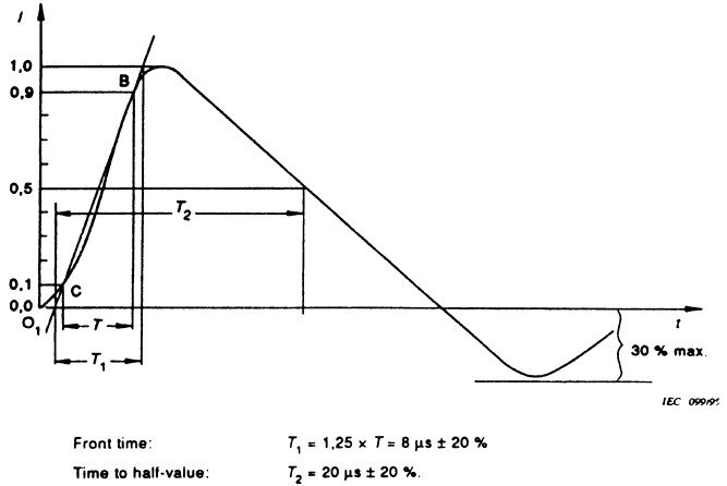
We will also examine scenarios wherein it becomes necessary to consider the influence of the Right Half Plane Zero (RHPZ) and the practical implications it entails. Once the components specific to the particular power supply are appropriately dimensioned, we can reasonably approximate the transfer function that mathematically describes the output power stage. As highlighted in the article “Find Poles and Zeros of a Circuit by Inspection“, will promptly identify the POLES and ZEROS characterizing the distinct switching categories.

The subsequent step involves generating Bode plots of these functions utilizing PSpice. Based on their characteristics, we will select the most suitable compensator G(s), implementing the compensation network through operational amplifiers integrated within the microcontrollers. Employing SPICE simulation on the open loop transfer function G(s)*H(s), we can assess the system’s stability outcomes.

Lastly, we will apply this methodology to two real-world switching power supply instances: a low-power flyback converter and an off-line, half-bridge switching configuration. This approach streamlines the design process for the compensator G(s) during the prototyping phase, preceding physical measurements with instrumentation.

It’s strongly recommended to read these articles first:

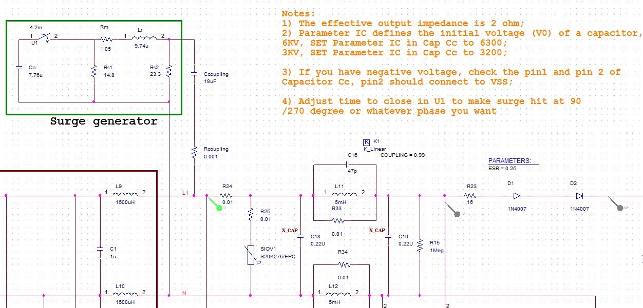
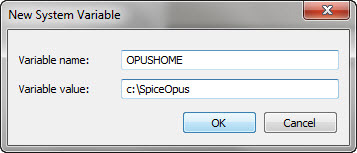
By accessing this article, you can download the following SPICE simulation files related to the design of compensation for switching power supplies:

-Forward function example

-Flyback function example

-Flyback function example with a Right Half Plane ZERO

-Origin POLE compensator

-Origin POLE Transfer function implementation

-Forward function compensated example

-One ZERO two POLES compensator

-One ZERO two POLES Transfer Function Implementation

-Flyback with RHPZ compensated

-Three POLES two ZEROS compensator

-Three POLES two ZEROS Transfer Function

-Transfer function of a real Flyback converter

-Compensator for the flyback converter

-Overall compensated transfer function of the flyback converter

-Transfer function of a real Forward converter

-Compensator for the Forward converter

-Transfer function of compensator for the Forward converter

-Overall compensated transfer function of the Forward converter

Premium Content

Pages: 1 2 3 4 5 6 7 8

Combination Wave Generator SPICE simulation.

In this article, we will delve into the implementation and analysis of a versatile Combination Wave Generator SPICE simulation template. This template forms the groundwork for a range of applications including Surge Generators, Line Impedance Stabilization Networks (LISN), motor control, and ripple current analysis. Hardware engineers can capitalize on this model to streamline project development efforts.While using PSpice for simulation, you can effortlessly apply the fundamental principles of the Combination Wave Generator SPICE simulation template to various other SPICE simulation software platforms.

A “Combination Wave Generator” finds its application in Electromagnetic Compatibility (EMC) tests, generating specific waveform voltage or current pulses. Its purpose is to assess electronic devices’ electrical resilience and responses to abrupt variations or transients within the electromagnetic environment. These generators replicate transient electrical disruptions or surges that might manifest in electronic circuits during situations like electrostatic discharges, switching transients, or line surges.

The Combination Wave Generator is an essential component of EMC compliance tests, ensuring that electronic devices can operate in realistic electromagnetic environments without sustaining damage or unforeseen behaviors.

Simplified SPICE Model of Combo Wave Generator.

The simplified model of the CWG consists of an High-Voltage source U, a charging resistor Rc, an energy storage capacitor Cc. This part of circuit is connected by a switch to 2 Pulse duration shaping resistors Rs, an impedance matching resistor Rm and a Rise time shaping indutor Lr, as in the picture below

typical values of this components are: Cc=7.76μF, Rs1=14.8 Ohm, Rm=1.05 Ohm, Lr=9.74μH, Rs2=23.3 Ohm. The peak voltage on Rs2 can be 1KV, 2KV,..6KV.

In the following schematic we set the high voltage with the initial condition of the CapacitorCc, for example for 6KV, we set 6300 in the PSpice IC field of the Cc component. We can adjust the time in U1 to make surge hit at 90/270 degree or whatever phase we want.

Calibration of Surge Generator.

The IEC/EN 61000-4-5 standars requires the following waveform of open-circuit voltage with no Coupling/Decoupling network (CDN) connected

This is the result of the simulation that shows a voltage waveform that fullfills requirementof IEC/EN 61000-4-5

Below the image of the waveform of short-circuit current with no CDN connected

and here again the simulated results:

Ipeak is about 1.5KA, T1 is 8uS and T2 is 20uS. The effective coupling impedance is 2Ohm. The simulated current waveform fulfills requirement of IEC/EN 61000-4-5 standards.

Pages: 1 2

Microcontroller-Based PID Controller Design and Simulation.

Ing. Cristoforo Baldoni

In this article, we will explore the transition from analog PID controller design for continuous-time systems to digital controllers, including PID controller simulation. This transition involves substituting operational amplifiers, resistors, and capacitors with microcontrollers. Digital controllers offer remarkable compactness, fitting the entire controller onto a single chip, complete with A/D and D/A converters. Furthermore, digital controllers remain immune to component aging and temperature-induced value fluctuations, in contrast to analog components.

We will delve into the application of the Z-transform, which serves as the discrete-time systems counterpart to the Laplace transform. This exploration will encompass the identification of a process’s transfer function. Through a systematic, step-by-step approach, we will demonstrate the practical application of theoretical insights. This will be accomplished by analyzing a Proteus microcontroller-based project, wherein the PWM output is harnessed to regulate the temperature of an oven. The microcontroller boasts a 10-bit A/D converter.

This adaptable procedure can be easily customized with minimal adjustments for controlling various other processes.

Topics Covered:

1. Digital Control-System Block Diagrams.

2. Linear Difference Equations, Z-Transform, Inverse Z-Transform and Discrete Transfer Function.

3. Sampling and A/D Conversion: Analog to Digital Converter.

4. D/A Conversion and ZERO ORDER HOLD (ZOH) : Relationship between the Continuous Transfer Function and Discrete Transfer Function of a Sampled Process.

5. Manipulation of Block Diagrams for Sampled Data.

6. Methods for designing Digital Controllers and Ensuring Stability.

7. Microcontroller-Based PID Controller Design.

8. Transfer Function Identification and PID Tuning using the Ziegler–Nichols Method.

9. Practical case of a temperature control system implemented with a microcontroller PIC and simulated with ISIS Proteus: Step by step explanation of how to apply the theoretical knowledge for implementing and simulating a PID controller.

Premium Content

Pages: 1 2 3 4 5 6 7

SPICE-Based Design of PID Controllers.

In this comprehensive article, we delve into the world of industrial control systems through the lens of PID controllers using SPICE simulation. We will embark on a journey to explore the process of designing and simulating various types of PID controllers – including Proportional (P), Proportional-Integral (P.I.), Proportional-Derivative (P.D.), and Proportional-Integral-Derivative (P.I.D.) controllers, leveraging the power of SPICE simulation. The article delves into the theoretical underpinnings and practical methodologies for creating these controllers, emphasizing their importance in optimizing diverse industrial processes. Additionally, we’ll take a closer look at the subsequent implementation of these controllers, achieved using operational amplifiers. Whether you’re an engineer, a researcher, or a technology enthusiast, this article offers valuable insights into the dynamic world of PID control and its application within industrial contexts.

Premium Content

Pages: 1 2 3 4 5

Find Poles and Zeros of a Circuit by Inspection

Ing. Cristoforo Baldoni

In this article, focused on ‘Poles and Zeros of a Circuit‘, we will explore the technique of identifying the count of poles and zeros within a transfer function, including those in complex linear networks, solely through visual inspection. This method obviates the need for calculating the analytical expression of the transfer function. By the conclusion of this article, you will have the capability to swiftly determine the number of poles upon initial examination.

Once the output is established, this approach also enables you to ascertain the quantity of zeros through inspection and subsequently compute the precise symbolic form of the transfer function. Additionally, you can calculate the exact values of both zeros and poles employing user-friendly software tools readily accessible for free. We will validate the findings using SPICE analysis.

The primary objective of this article is to delve into the concepts of poles and zeros within a transfer function, elucidating their physical significance. Furthermore, we aim to furnish valuable analytical tools to aid analog circuit designers and control systems engineers in their endeavors.

How many POLES does this circuit have?

And how many does this high-pass filter have?

If your response to the initial question is 9 or 8, or if you do not identify a fifth-order filter (with five poles) in the filter’s illustration, then you should proceed to read this article.

Premium Content

Pages: 1 2 3

Control Systems using SPICE Simulation.

Ing. Cristoforo Baldoni

Exploring the domain of Control Systems using SPICE Simulation, this article offers essential principles for designing and analyzing Feedback and Control Systems. Control Systems theory, a cornerstone of engineering and automation, involves the study of dynamic systems and their manipulation to achieve desired outcomes. These systems are omnipresent in our modern industrial technological world, seamlessly integrated into everyday devices. They play a vital role in processes as diverse as the precise positioning of a Reader’s laser, the intricate control of a hard disk head’s movement, and even the numerous biological control systems orchestrating our bodily functions.

Control Systems theory involves understanding how systems respond to various inputs and disturbances, and how to design controllers that shape these responses to achieve desired goals. These goals can include stability, accuracy, speed, and overall performance optimization. Whether it’s managing the temperature of an oven, stabilizing the flight of an aircraft, or controlling the speed of a motor, the principles of Control Systems theory provide the framework to analyze, design, and optimize these dynamic processes.

As we navigate through this article, we’ll begin by introducing the basic concepts that underpin Control Systems theory. From there, we’ll seamlessly transition into exploring how these theories come to life through the application of SPICE simulation. Our journey includes the evaluation of the Open Loop Transfer Function using the versatile tool of PSPice, providing hands-on insights into the practical implementation of control strategies. Whether you’re a novice eager to comprehend the foundations or an enthusiast seeking to refine your expertise, this article offers a holistic perspective on the symbiotic relationship between Control Systems theory and the power of SPICE Simulation.

Topics Covered:

1. Processes, Open Loop and Closed Loop Control Systems (Feedback Systems).

2. Generic Closed Loop Schematic of Feedback Systems.

3. Physycal Processes Modeling, Differential Equations and Laplace Transform Simplification.

4. Transfer Function: Understanding Poles, Zeros and their Phisical Significance.

5. Natural and Forced Response: Residues Calculation, Simplification of identical Zeros and Poles, Dominant Poles.

6. Process Stability.

7. Steady State Erro and Systems Types.

8. Transfer Function through Bode Diagram Analysis. Examination of the Open Loop Transfer Function using SPICE Simulation.

Premium Content

Pages: 1 2 3 4 5 6

Getting Started with PyOPUS

PyOPUS is a Python based platform for very sophisticated circuit optimization and simulation automation. It represents a library designed for optimizing arbitrary systems through simulation. Its primary focus is on refining circuit performance. Serving as the foundation for the PyOPUS GUI, this library facilitates the effortless configuration of design automation tasks. Within the GUI, users are also able to visualize outcomes and graph the waveforms produced by the simulator.

The module labeled “pyopus.simulator” presently offers compatibility with SPICE OPUS, Ngspice, Xyce, HSPICE, and SPECTRE. The use of the Python library with the simulator requires a previous SPICE OPUS (or other SPICE software compatible) installation, then refer to the relative tutorial before proceeding.

Now let’s see how to install PYOPUS on Windows. The download page offers software for Linux and Windows platforms, but discontinues 32-bit Windows support due to the unavailability of the 32-bit Windows SciPy wheel.

Python	Programming language
NumPy	Package for scientific computing with Python
SciPy	Python software for mathematics, science, and engineering
MatPlotLib	Python 2D plotting library
wxPython	Blending of the wxWidgets C++ class library with Python
PyOPUS installer	the Windows PyOPUS installer

All these softwares can be downloaded here

Let’s start with the Python installation

the default destination directory is C:Python26

the full features installation requires about 50MegaByte

after the installation we have to add an enviroment variable: Start/Control Panel/System and Security/System/Advanced system settings, now click on Enviroment Variables button.

add to “Path” variable the value “C:Python26”

Pages: 1 2 3

SPICE OPUS Circuit Simulation

SPICE OPUS, an acronym for SPICE engine for OPtimization UtilitieS, represents a powerful circuit simulation tool. This software is a recompilation of the original Berkeley’s source code, designed to work seamlessly on Windows 95/98/NT and Linux operating systems, supplemented by Georgia Tech Research Institute’s XSPICE mixed-mode simulator.

With SPICE OPUS, you have the capability to perform simulations on a wide range of circuit types, including analog, digital, and mixed-signal configurations. This versatile tool is available for both Windows and Linux platforms, although it does not feature an integrated schematic program for component selection and circuit drawing.

Developed by the Faculty of Electrical Engineering at the University of Ljubljana, Slovenia, SPICE OPUS has gained substantial recognition worldwide, amassing a user base of over 10,000 individuals spanning various domains such as research, education, and industry.

Throughout this article, we will guide you through the straightforward process of installing SPICE OPUS on a Windows environment. Additionally, we’ll delve into the procedure for describing a circuit to simulate, achieved by crafting a .cir file using a standard text editor.

You can download the updated software here

After downloading the program run the Setup.exe

Installation on Windows

you can change the installation directory by clicking on Browse button, by default it is installed in C:SpiceOpus

when the setup is complete, open the Start menu and go to Control Panel, choose “System and Security” and again “System”, once open this window, click on “Advanced system settings”

the “System Properties” window pops up:

click on “Enviroment Variables…”

Add a new system variable by clicking on the lower “New” button.

Name the variable OPUSHOME. The specified directory must be the Spice Opus installation directory. Click on OK. Confirm your changes by clicking on OK in the Environment variables dialog and once more in the

System Properties dialog.

Installation on Linux

Become root.

su –

Unpack the .tar.gz archive.

A directory will be created with the name that looks like

spice_opusXXX_linux_DATE_TIME

Enter this directory.

cd spice_opusXXX_linux_DATE_TIME

Start the installation script (spice.install).

./spice_install INSTALL_PREFIX

INSTALL_PREFIX is the tree where Spice Opus will be installed. The recommended location is

/usr/local. The installation script removes any previous Spice Opus installation in that tree and

replaces it with the latest version. The binaries go to INSTALL_PREFIX/bin .

After the installation is finished, you can remove the spice_opusXXX_linux_DATE_TIME

directory that was created by unpacking the .tar.gz archive.

Setting up the environment.

We shall assume that you are using BASH. Add the following two lines to /etc/profile (you

must be root in order to be able to do it).

OPUSHOME=INSTALL_PREFIX

export OPUSHOME

where INSTALL_PREFIX is the tree where you installed Spice Opus.

It is also convenient if you add INSTALL_PREFIX/bin to your path. Add the following two

lines at the end of /etc/profile.

PATH=$PATH:$OPUSHOME/bin

export PATH

Log out and log in again for the changes to take effect.

Pages: 1 2 3

Altium Designer Video tutorials

This page serves as a valuable resource, offering a curated collection of YouTube videos that explore what Altium Designer can do. These tutorials have been chosen to facilitate a swift learning curve, catering to both novices and seasoned designers alike under the banner of “Altium Designer Video tutorials.”

The videos featured here span a wide spectrum of topics, encompassing various types of analyses within SPICE simulations. Whether you’re interested in DC, AC, transient, or frequency-domain analysis, these tutorials provide insightful guides on each facet. Furthermore, the page delves into the intricate journey of PCB design, walking you through the different stages from initial schematic layout to the final Gerber files.

From schematic capture to footprint selection, netlist generation to component placement, and routing to design rule checks, these videos intricately navigate through the entire design process, ensuring a comprehensive understanding of Altium Designer’s capabilities. Whether you’re a seasoned professional aiming to augment your skill set or a newcomer navigating the world of PCB design, this collection will undoubtedly prove to be an invaluable asset. Explore the world of “Altium Designer Video tutorials” and unlock the full potential of SPICE simulation and PCB design.

Topic	Video
Getting started with Altium Designer
Installing SPICE Simulation Libraries
Find Devices with SPICE Simulation Models
Configuring SPICE Simulation Parameters
SPICE Templates for Devices
Direct SPICE Model Editing
SPICE Netlist from Schematic
Link a SPICE PSPice XSPICE simulation model to a schematic symbol
Waveform Editor
SPICE DC Sweep Analysis
SPICE AC Sweep Analysis
SPICE Operating Point Analysis
SPICE Transient Analysis
SPICE Monte Carlo Analysis
Fourier Analysis
Parameters Sweep in SPICE Analysis
Getting Started with PCB Design
Schematic Design
Schematic Symbols
PCB Footprint and 3D model
Mounting Holes
Importing Librarian Parts
Part Libraries
Variants DNP
Bill Of Material
PCB Layout Setup
Ground Plane
PCB Fanout to Copper Plane
Routing
Silkscreen and PCB Notes
Gerber Files
Documentation
From 0 to Gerber

An interesting and current vide o is the one that explains how ChatGPT can be helpful in printed circuit board design.

Altium Designer SPICE simulation

Dive straight into the world of Altium Designer’s SPICE simulation with practical ease. In this instance, we will walk through the creation of a dual-supply inverting operational amplifier circuit. Leveraging the robust capabilities of Altium Designer’s SPICE simulation tools, we’ll lead you through each phase of the process, enabling you to efficiently design and simulate the circuit’s performance. This hands-on experience offers valuable insights into the realm of Altium Designer SPICE simulation, enhancing your circuit analysis and design skills.

On this page, you can discover additional resources to delve deeper into the possibilities of SPICE simulation and learn how to create the PCB for a circuit using Altium Designer.

Let’s begin with the creation of a new circuit schematic.

a new blank sheet pops up

on the top toolbar we find the icon to place part

The place part window appears

Siglent Technologies SDS1202X-E 200 mhz Digital Oscilloscope

Click on the button “…” to open the Browse Libraries window

moving throughout the first list we can select a library

Once selected the library we can easily choose a library’s component

Pages: 1 2 3 4 5 6